// Data visualization

Spring Shipping Season

Showing where and when produce season tightens truck capacity, as the harvest moves from southern markets to northern ones.

Role
Data analyst, visualizer, and subject-matter expert
Timeline
Spring 2023
Tools
Tableau
Team
Design and marketing colleagues
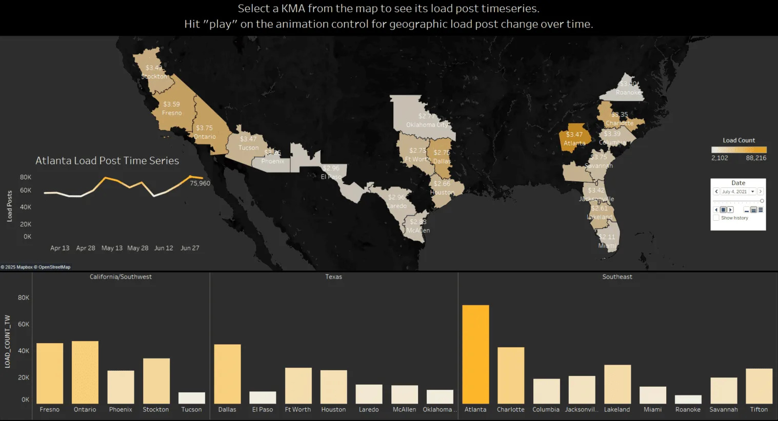
A Tableau dashboard on a dark background. A map of the southern US shades California, Texas, and Southeast freight markets by load count, with Atlanta darkest, and labels each market's rate per mile. An inset line chart shows Atlanta's load posts from April to late June, ending at 75,960. Below, bar charts compare load counts by market in three regions: California/Southwest, Texas, and Southeast.(opens full size)
The animated load-post dashboard. Press play to watch load posts shift across markets over the season. Select a market to see its load-post time series.

Overview and objective

On this project I was the data analyst, visualizer, and subject-matter expert in a cross-team collaboration with design and marketing. The message they wanted the marketing collateral to carry: tell readers when and where freight capacity will be tight.

My goal was to tell the story of produce freight ramping up during the spring growing season, April through July. I wanted to show how that freight travels from southern markets to northern ones, and how it tightens capacity along the way.

Exploration and iteration

The team wanted to know whether a joy plot would work for this story. I built a few trials in Tableau and presented them to the team. Each ridge is an outbound freight market, with load activity plotted over time along the x-axis.
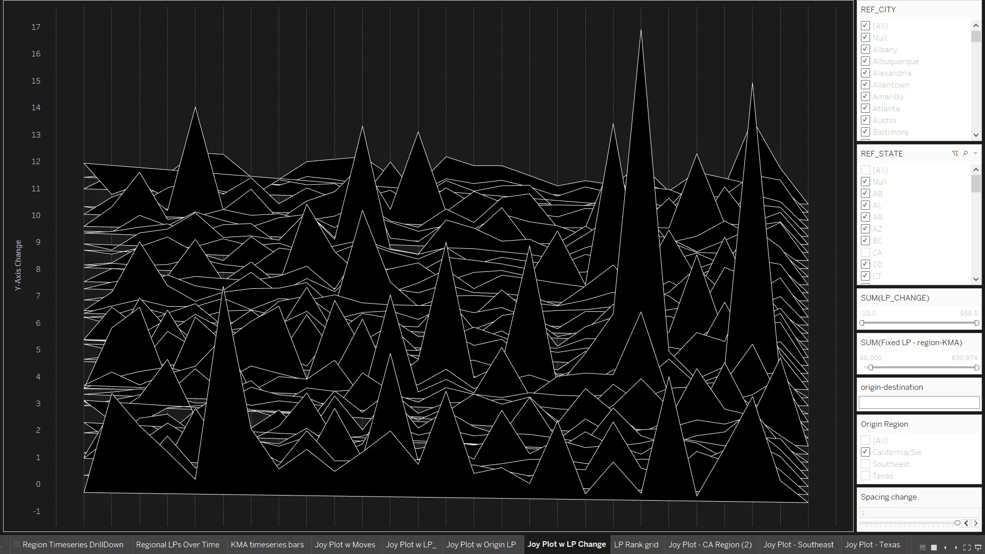
A black-and-white joy plot in Tableau: dozens of overlapping white-outlined ridges, one per freight market, with sharp peaks of varying height. Filter panels for city, state, and origin region sit on the right.(opens full size)
Iteration 1: the change in load posts for every market, stacked as ridges.
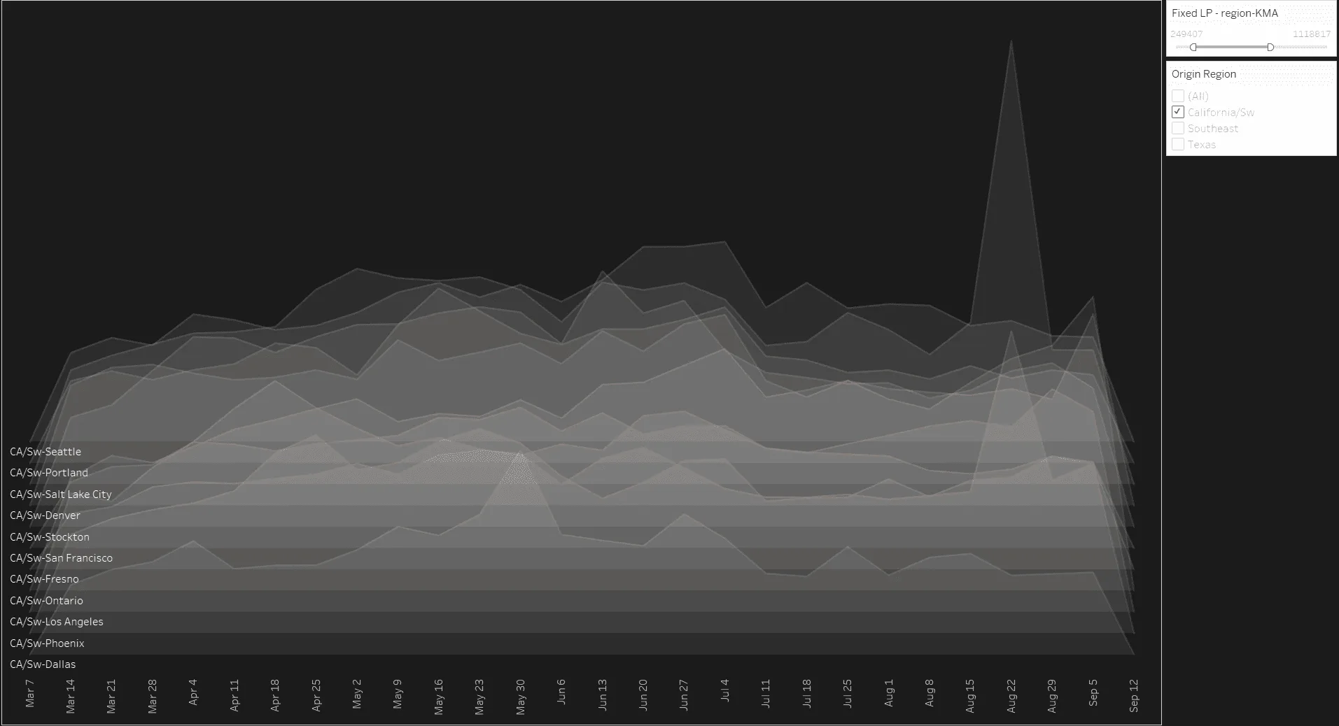
A softer gray joy plot in Tableau: eleven translucent ridges labeled California/Southwest markets, from Dallas at the bottom to Seattle at the top, plotted weekly from March 7 to September 12.(opens full size)
Iteration 2: California and Southwest markets only, March through September.

The joy plots were fun to create, but they didn’t show the south-to-north movement over time clearly or concisely enough to land the message with our audience. Once I added color, the trends we wanted to show readers started to appear.
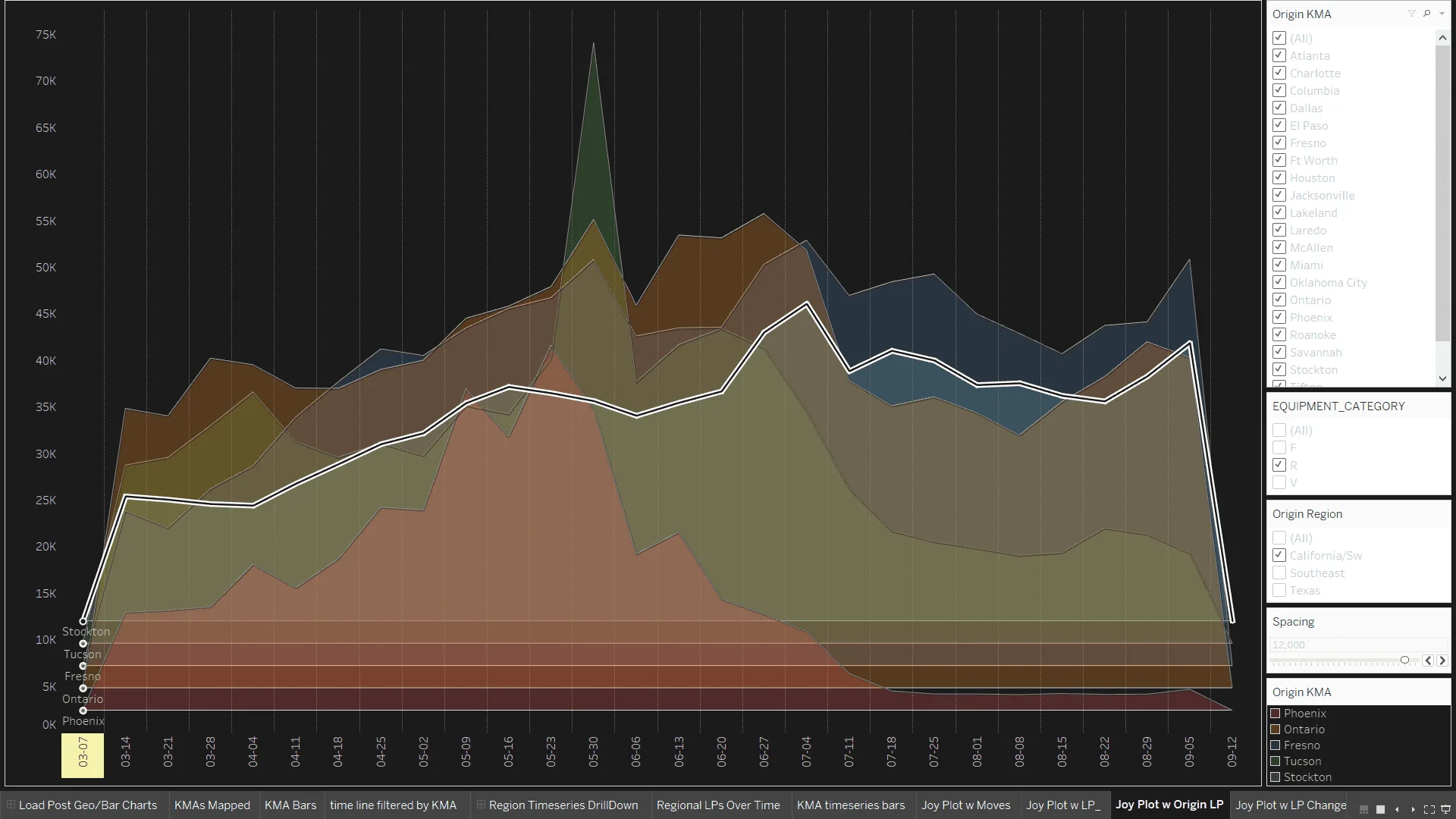
A layered area chart in Tableau with one colored band per market (Phoenix, Ontario, Fresno, Tucson, and Stockton) from March to September. A white line traces the total, rising from about 12,000 to peaks near 45,000 in early July and early September. A red band peaks in late May and then falls away.(opens full size)
Demand over time in California-region markets, plotted south to north from bottom to top.

Final design

From there, I built an animated dashboard, shown at the top of this page, for the teams to reference while they created the final collateral. I rolled it out to these internal stakeholders with a short walkthrough presentation.

A design colleague created the final piece: a two-page white paper published in spring 2023. It was used as marketing collateral and in a blog post on produce shipping season.
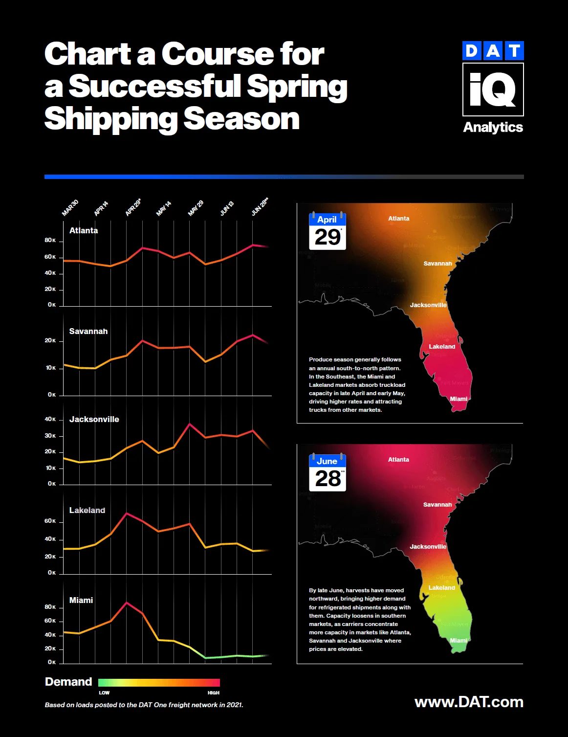
Page 1 of a DAT iQ white paper titled 'Chart a Course for a Successful Spring Shipping Season.' Line charts show demand from March to June for Atlanta, Savannah, Jacksonville, Lakeland, and Miami, colored from green (low) to red (high). Two heat maps of the Southeast compare April 29 and June 28: demand is concentrated in Miami and Lakeland in spring and moves north to Atlanta, Savannah, and Jacksonville by late June.(opens full size)
Page 1 of the final white paper, designed by a design colleague.