Workflow Optimization: Putting a New Metric to Work

Overview and objective

In 2022, the marketing team asked me to help our users understand the Market Conditions Index (MCI), DAT’s capacity metric: how to think about it in terms of freight rates, and how to use it. MCI rates each Key Market Area with a capacity score from −100 (loose) to 100 (tight). A data scientist on another team developed the metric, so I spent the fall researching it, listening to the data scientist explain how it was built, and then building the talk-track for using it. The result of that research was my first conference talk, a product lab at DATCon 2022.

After that presentation, a salesperson paired me with a customer partner at a small-to-mid-sized brokerage. My team was very familiar with the data needs of large brokers and wanted to learn the needs of brokers like this one, so it was the right opportunity to learn from the customer. The salesperson and the customer partner both felt there had to be a way to use MCI with pricing data to finesse a rate decision on a given lane. I took their request to pair MCI with rate data and came back with the Benchmarking with MCI dashboard concept.

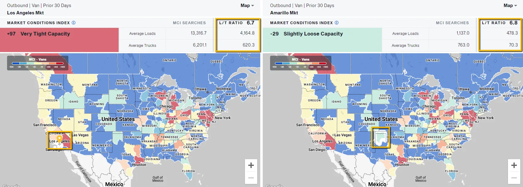
My 2022 talk set out what MCI is and why a capacity score adds something a ratio can’t. Two markets can show almost identical load-to-truck ratios and be very different markets. MCI is cleaned and geographically normalized, so it lets a headhaul market and a backhaul market be compared directly.

Two side-by-side DAT market views for outbound vans over the prior 30 days. Los Angeles has a load-to-truck ratio of 6.7 and an MCI of +97, Very Tight Capacity. Amarillo has a ratio of 6.8 and an MCI of −29, Slightly Loose Capacity. Both ratios are boxed in yellow, and below each, a US map colors markets from blue (loose) to red (tight). — From the 2022 talk: almost identical ratios, very different markets.

Exploration and iteration

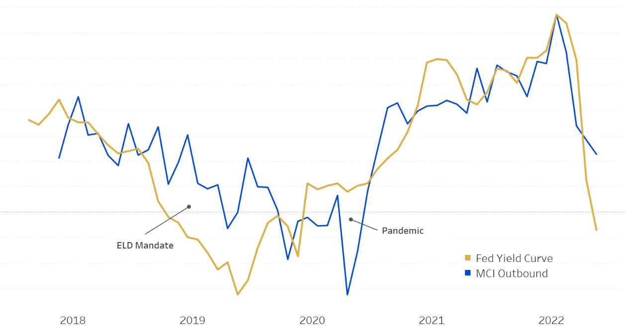
I also revisited how MCI tracks the broader economy. Lagged three months, national MCI correlated with the Federal Reserve yield curve at .78 in my 2022 analysis. When I updated the chart in spring 2023 it was .68, still strong. The freight market has been in an unprecedented recession since then. I believe 2023 was the start of it, so that falling number was an inflection point, with prices falling and continuing to fall through 2025.

A line chart from 2018 to 2022 comparing the Fed yield curve (gold) with outbound MCI (blue). The two lines dip together through 2019, with the ELD mandate and the pandemic annotated, climb together through 2021, and both drop sharply in 2022. — National outbound MCI, lagged three months, against the Federal Reserve yield curve, 2018 to 2022.

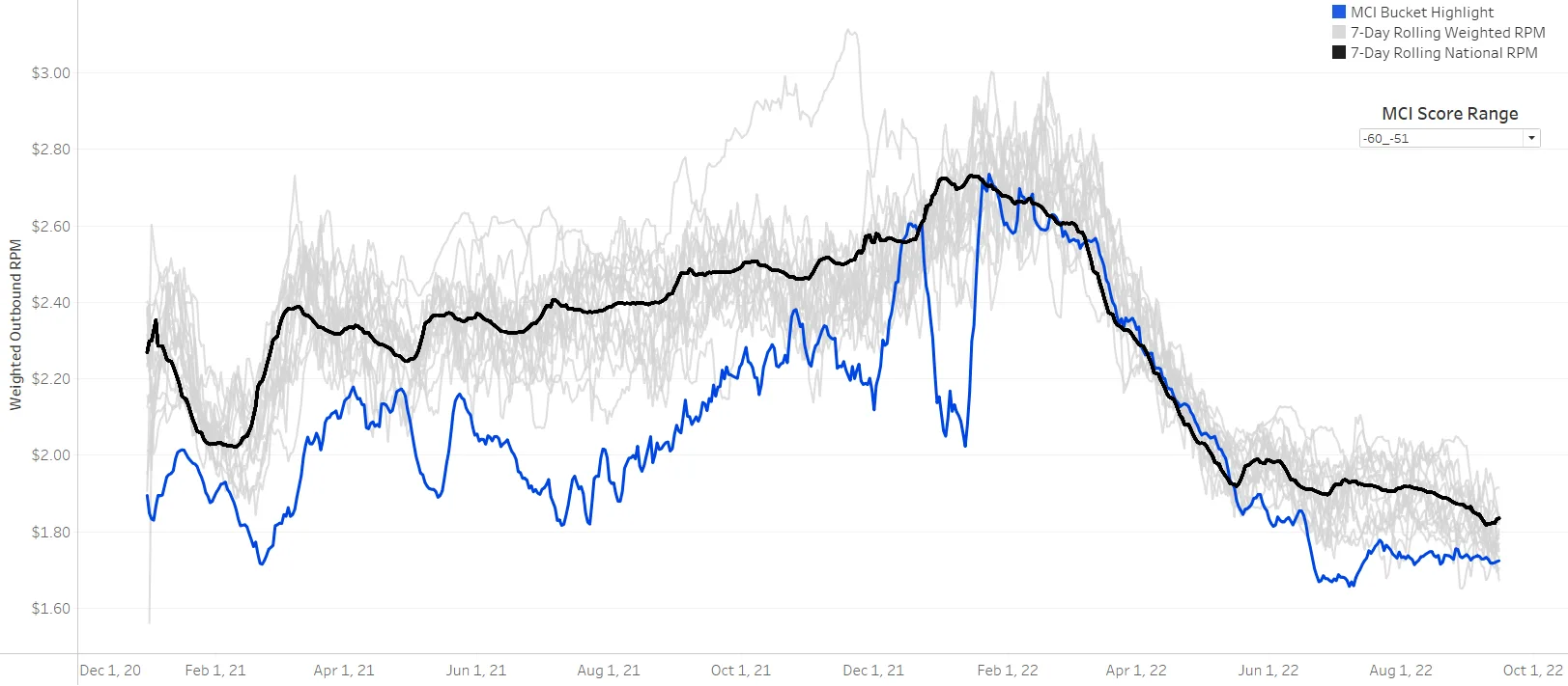
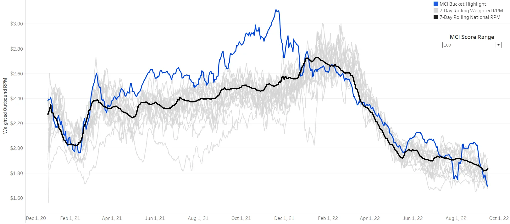
The finding that set the direction came from bucketing outbound rates by MCI score. Nationally, loose capacity lanes tend to be priced below the national average and tight capacity lanes above it. The markets MCI defines as looser appear to have more negotiating power. After being tasked to develop a talk-track around MCI and socialize the product, I wanted to start applying the metric to real customer workflows, and to see if this broad national analysis could translate to a customer’s own network.

A line chart of weighted outbound rate per mile from December 2020 to October 2022. Gray lines show every MCI bucket and a black line shows the national average. The highlighted blue line, for MCI scores of −60 to −51, runs below the national average for most of the period. — Loose markets (MCI −60 to −51) priced below the national average.

The same line chart with the MCI score range set to 100. The highlighted blue line runs above the national average for most of 2021, peaking above three dollars a mile in late 2021. — Tight markets (MCI 100) priced above it.

The proof-of-concept visual began to take shape one morning when our Chief of Analytics asked me to describe what MCI is: let’s use MCI to apply nuance to a rate’s situation. Should a customer have paid over the market rate on those lanes? Maybe it was warranted, because they were coming out of tight markets. But we needed a working relationship with a customer to tell us if we were, as one of our Directors of Product puts it, solving a problem “from the inside out.”

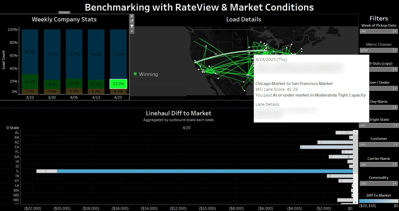
I first reproduced the national chart at the customer level, benchmarking the customer’s rates against their own network average. And we found something interesting. The rates they paid to move loads out of loose capacity markets trended higher than their network average. That was an anomaly, since the national analysis said rates out of loose markets should trend below. I added a hover layer showing which outbound markets those loads came from, and the customer partner started to recognize the areas right away. His gut reaction confirmed these may be markets to focus their buying strategy or improve their carrier network.

A line chart on a black background from February 14 to March 16. A white line shows the customer's network rate, blue lines show each MCI bucket's 7-day rolling rate, and one highlighted gold line, a loose-capacity bucket, runs well above the network rate for most of the period. — The customer-level version. Rates out of loose markets (gold) trended above the customer's network average (white). The chart title, which named the customer, is cropped.

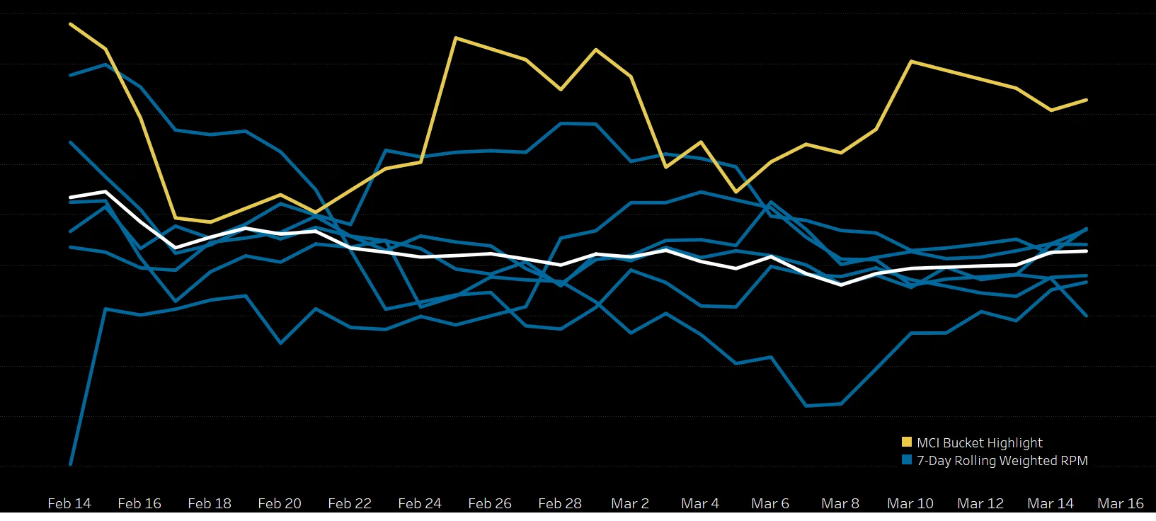
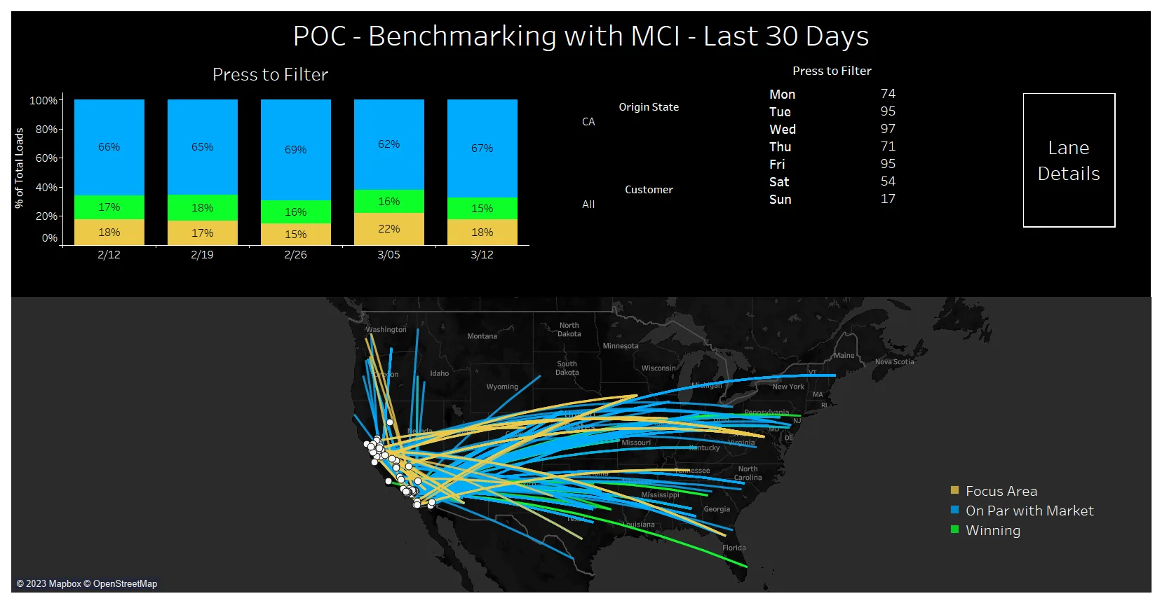
From there, we decided to test a lane-based MCI score in historical benchmarking. Pairing each lane the customer ran with its best-match RateView market rate, I added an MCI lane score, so the analysis could go past “we paid over” or “we paid under” to the conditions the rate was paid in. Our two teams met on a regular cadence to review the visual, the edits they wanted, and their questions. I co-presented the proof of concept with the customer partner at a learning lab at the TIA Capital Ideas Conference in spring 2023.

A Tableau dashboard titled 'POC – Benchmarking with MCI – Last 30 Days.' Five weekly stacked bars split loads into three categories, with most loads in On Par with Market and smaller shares in Winning and Focus Area. Beside them, filters and a count of loads by day of the week. Below, a dark US map draws the customer's lanes in the three category colors, most of them running east out of California, with a legend for Focus Area, On Par with Market, and Winning. — The proof of concept, co-presented at TIA Capital Ideas 2023.

A conference learning-center stage with a TIA 2023 Capital Ideas Conference backdrop. A screen reads 'Our Ongoing Collaboration' above a dashboard thumbnail. Kassondra stands near a podium talking with a man, while two other attendees stand at a high-top table facing the screen. — The learning lab at TIA Capital Ideas 2023.

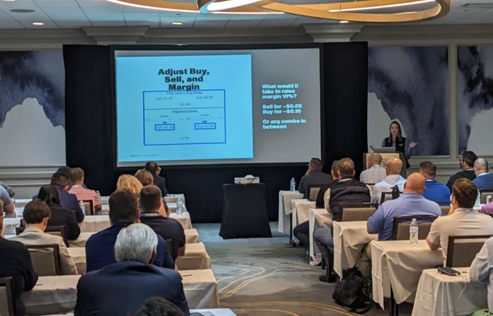
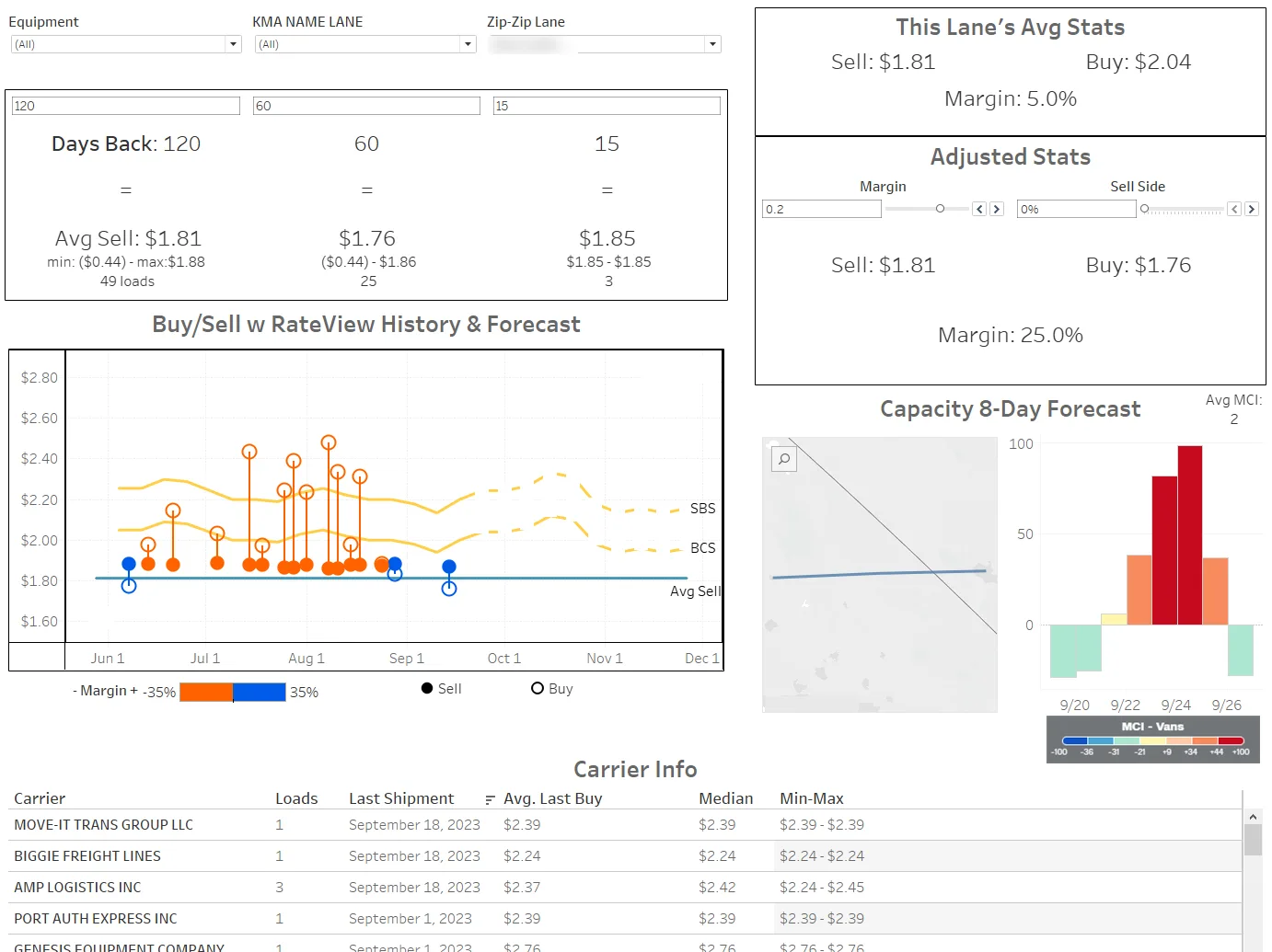
Through 2023, the work kept evolving into Blue Sky Margins, which I presented at DATCon 2023. It reversed the order of the analysis: first it drilled into a broker’s lane-level margin that sat below the industry average, then it ran the benchmarking-with-MCI analysis on those lanes, drilling into lanes where the rate paid was above market in areas where capacity was loose. It added the sell side, margin adjustment, rate and capacity forecasts, and the carriers who had recently moved loads on the lane.

Kassondra presenting at a podium in a hotel ballroom to a full room of seated attendees. The projected slide, 'Adjust Buy, Sell, and Margin,' shows the lane's average and adjusted stats and asks what it would take to raise margin 10%: sell for about $0.05 more, buy for about $0.10 less, or any combination in between. — Presenting Blue Sky Margins at DATCon 2023.

Key decisions

Leading the user to the conclusion. I chose against DAT’s standard practice of presenting data and letting RateView users draw their own conclusions about their position to the market. Instead, I lead the user to conclusions through the analysis, so that instead of their next action being more analysis, their next action is acting on the lanes that weren’t priced effectively for profit.

Three categories instead of two. I decided on the categories. They replaced the simpler “over market” or “under market” result of straight benchmarking to the market rate, without capacity context:

Winning: paid at or under market in tight capacity
Focus Area: paid over market in loose capacity, meaning they overpaid out of and into markets where they most likely could have sourced capacity for a lower price. This is what to look at first.
On Par with Market: everything else, including paying over in tight markets or under in loose ones, where the variance to market was warranted

Where “over” starts. A load only counts as over or under market when it is at least $50 and at least 5% off the market linehaul rate. I arrived at those cutoffs by talking with the customer partner, then ran them by other brokers who purchased the dashboard, and they agreed it worked for them.

Final design and outcome

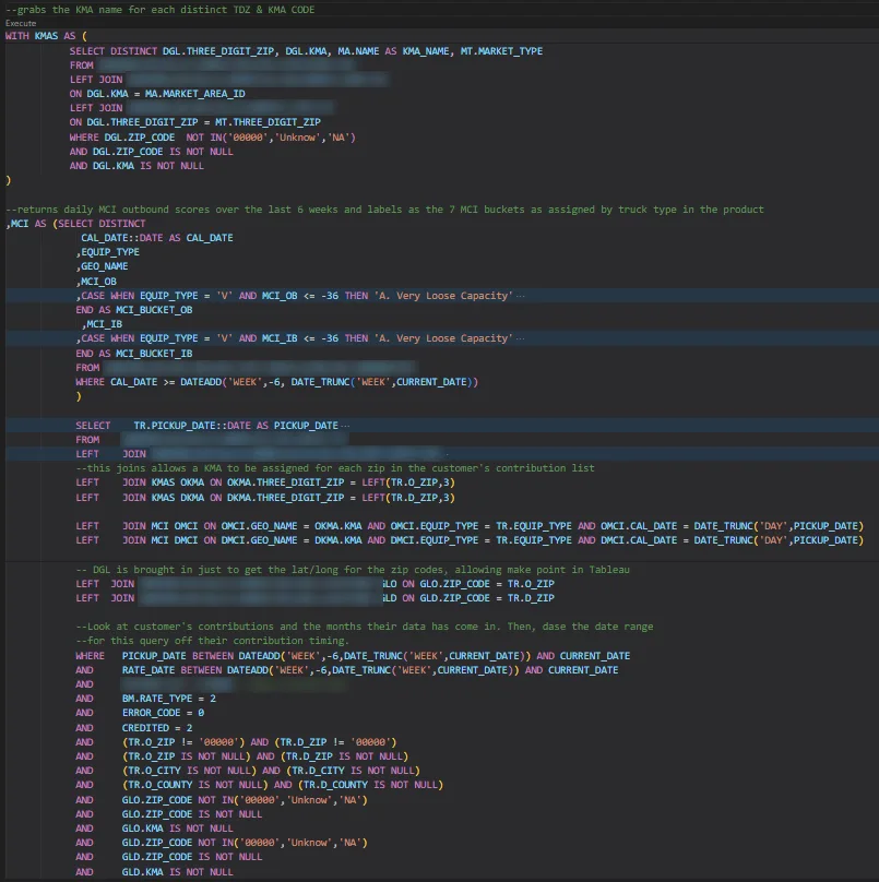
A custom SQL script powers the dashboard, with the calculations written into the query itself. It labels daily capacity scores into seven buckets from very loose to very tight, by truck type, and joins the customer’s rates to those scores by origin, destination, equipment type, and pickup date. I developed the calculations after hearing how customers wanted to use the metric.

A SQL script in a dark code editor. Common table expressions look up market names for each three-digit ZIP code and label daily capacity scores into seven buckets, from very loose to very tight, by truck type. The main query joins a customer's rates to those scores by origin, destination, equipment type, and pickup date for the last six weeks. Database and table names are blurred. — Part of the custom SQL behind the dashboard. Database and table names are blurred.

The customer partner used the dashboard on a weekly basis to focus his carrier sales team on areas where they could be buying capacity at a lower rate. The analysis gave them specific lanes, origins, and destinations where the team could focus on either sourcing better or negotiating tighter. He reported that the dashboard let him successfully focus the team and bring paid rates down.

The outcome: Benchmarking with MCI was set up for 25 customers. In 2024 our carrier salesperson for Key accounts sold it as part of a package deal to new and upgrading carriers and broker/carriers. The full lane-based capacity analysis wasn’t built into DAT’s product, but an origin-and-destination version was included in 2024 as v2 of DAT’s newly released benchmark analytics product, and I was a source for how to apply MCI to benchmarking analysis.

Blue Sky Margins got great feedback and excitement during the talk, but it didn’t take off in customer demo calls afterward. The feedback I received was that brokers didn’t want DAT to analyze their margin, and dashboards built around margin weren’t welcome as a product to buy from DAT.

A light Tableau dashboard for a single lane. Top left, average sell rates over the last 120, 60, and 15 days. Top right, the lane's average sell, buy, and margin, with sliders to adjust margin and sell side. Middle, a buy and sell chart plots loads against RateView history and a dotted forecast. Right, an 8-day capacity forecast in MCI colors. At the bottom, a Carrier Info table lists recent carriers with load counts, last shipment dates, and rates. The lane is blurred. — Blue Sky Margins, presented at DATCon 2023. The lane is blurred; the carrier names are sample data.

Reflection

As I moved into a managerial role, my direct report took over standardizing the dashboard. We needed a version of the file that could be set up quickly for new customers. If I were to do this project over again, I would have been cleaner about my Tableau calculated fields and kept a glossary of what each field was, how they worked together, and how each one contributed to the analytics on screen.

Blue Sky Margins was the other key learning. I believe that if DAT’s analytics product incorporated margin analytics, brokers would take to the idea, especially with in-app privacy messages reminding users that their company-specific analytics are never shared with other customers. That belief still needs user interviews and testing to prove.